The form of the line is
y = mx + b, where m is the slope of the line and b is the y intercept.The formula for m is:
Sum(xi*yi) - n*xavg*yavgSince just one x and y specify just one point, we will use two arrays: one to hold the x-values and one to hold the y-values.
m = ------------------------ ,
Sum(xi2) - n*xavg2
where n is the number of points in the data set.
The formula for b is:
b = yavg - m*xavg
Continuing with our global warming example, if a scientist comes up with the square of the correlation at 0.999, this means that she can predict very accurately how fast the earth is warming. If she comes up with a square of the correlation at only 0.256, the data doesn't accurately predict how fast the earth is warming.
The formula for the square of the correlation is:
        (n*Sum(xi*yi) - Sum(xi) * Sum(yi))2
r2 = -----------------------------------------------------
        (n*Sum(xi2) - Sum(xi)2) * (n*Sum(yi2) - Sum(yi)2)
| n | X | Y | X2 | Y2 | X*Y | |
|---|---|---|---|---|---|---|
| 1 | 186 | 15.0 | 34596 | 225.0 | 2790 | |
| 2 | 699 | 69.9 | 488601 | 4886.01 | 48860.1 | |
| 3 | 132 | 6.5 | 17424 | 42.25 | 858 | |
| 4 | 272 | 22.4 | 73984 | 501.76 | 6092.8 | |
| 5 | 291 | 28.4 | 84681 | 806.56 | 8264.4 | |
| 6 | 331 | 65.9 | 109561 | 4342.81 | 21812.9 | |
| 7 | 199 | 19.4 | 39601 | 376.36 | 3860.6 | |
| 8 | 1890 | 198.7 | 3572100 | 39481.69 | 375543 | |
| 9 | 788 | 38.8 | 620944 | 1505.44 | 30574.4 | |
| 10 | 1601 | 138.2 | 2563201 | 19099.24 | 221258 | |
| Total | 6389 | 603.2 | 7604693 | 71267.12 | 719914.4 |
The first three columns represent our data. The right three columns represent calculations we do on the data.
Using the sums of X and Y we can quickly calculate the averages:
n = 10
Xavg = 6389/10 = 638.9

Yavg = 603.2/10 = 60.32
Using the sums in the table and the averages we can find all our statistics:
       719914.4 - 10 * 638.9 * 60.32
m = ----------------------------------- = 0.094962425
          7604693 - 10 * 638.92

b = 60.32 - 0.094962425 * 638.9 = -0.351493739
Our equation becomes:
y = 0.095 x - 0.3515
This equation takes the number of lines of code as its input and predicts how long it will take this student to finish the program. For example, if the program is 200 lines long, then
y = 0.095 * 200 - 0.3515 = 18.64or 18.64 hours.
The correlation squared is:
(10*719,914.4 - 6389*603.2)2r2 = 0.9107 tells us that the size of the program is a very good indicator of how long it will take the student to finish the project.
r2 = --------------------------------------------- = 0.9107
(10*7604693 - 63892)*(10*71267.12 - 603.22)
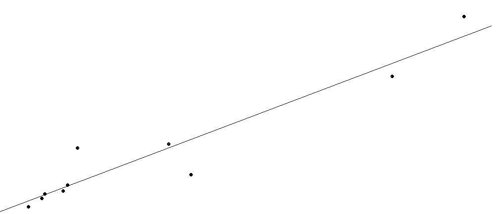
If we graph the data points and
the line, we see that the line goes right through the "middle" of the
collection of points.
Linear regression can be used for all sort of predictions.
Finally, many real world phenomena are do not follow linear trends. For example, the earth's population in recent history has been growing exponentially, not linearly. There are other mathematical modelling techniques available to help make these predictions. In reality, the math to match a exponential curve to data is very similar to what we have done here.